Mass-spring-damper

Mass-Spring-Damper Simulation

Introduction 

The mass-spring-damper problem is the simplest problem used in analysis of linear vibration. This example shows how to use the "classic" interface in MOMDYN to define the kinematics of the oscillator, and simulate its free vibration response.

Procedure

Using the classic interface, you will specify system constants (mass, stiffness, damping, and equilibrium length of the spring), a single generalized coordinate (vertical position), and use these to create a vector from the origin to the mass, a point, a particle, and the spring-damper. At completion, you will simulate the oscillating mass and visualize it's dynamics

Specify settings for the new model

Open MOMDYN, and tap once in the center of the screen to display the welcome screen. Tap the "Create" button, which will open the settings menu.

With the settings menu open, you can tap on each line item to bring up either a text input dialog, or a dropdown menu, for each respective item. This is used to modify their value, which is shown as the second text line for each item. Specify settings for the new model as follows:

• model_name: MassSpringDamper
• model_description: Common oscillator in vibration analysis

The "model_name" will be the name of the file if you choose to save the model. In this case, the saved pendulum model would display as user.MassSpringDamper if you were to save and then tap the "Import" button on the welcome screen. The "model_description" is solely for informational purposes.

• gravity_method: Uniform
• gravity_constant: 9.8
• gravity_direction: -Y

Gravity can be modeled either as "None" or "Uniform," where in the latter case gravitational force on each body is equal to its mass times the "gravity_constant" value. The gravitational force vector is given by the "gravity_direction" value.

• time_duration: 10.0
• simulation_rate: 100.0

The above values are used in simulation of the system. The "time_duration" in seconds is the total length of the simulation, and "simulation_rate" in Hertz (Hz) is the number of sample points per second in the output dataset if using a fixed-step solver , or initial step size if using an adaptive step solver.

• simplify_equations: False
• integration_method: RKF45
• tol: 0.001

The "simplify_equations" is useful for more complicated models, where trigonometric identities can be used to reduce the overall complexity, but tends to require more up-front computational time. The default "integration_method" is Runge-Kutta-Fehlberg (RKF45), and uses an adaptive step size with tolerance 0.001. Using smaller tolerances will generally reduce the step size and yield a more accurate simulation, but will increase computational time.

Tap the "check" button in the lower right to close the settings menu and create the new model as-specified above.

Create parameters (constants)

After closing the settings dialog, the screen will shift to the diagram view, with a single point representing the origin marked "O," and the inertial reference frame represented by the basis vectors (i, j, k).

Tap the menu button (three horizontal lines) in the lower right to obtain the menu dialog. Note the settings button in the upper left which will open the previous dialog, in case you want to edit any of the previously generated settings. The save button will save your model for future use, where it will be accessible using the import button on the first screen.

Tap on the panel labeled "Classic," which will expand to show several component options, each with four buttons, a "plus" to add a parameter, a "minus" to delete a parameter, a button to edit an existing component, and a question mark icon to view the help.

We will create parameters for the mass, and stiffness, damping, and equilibrium length of the spring. Tap the plus symbol on the parameter line to open a "New Parameter" dialog. The "name" line item will be the symbol given to the parameter, The value is the numeric constant for that parameter, and the description is short text describing its usage. 

We will use the name "m" for mass. Enter 1 for the value. Descriptions are optional, but recommended to include, as I have done below. Tap the check mark in the lower right to create the mass with specified parameters.

Once again, tap the plus sign in the Parameter panel, and repeat the above process three times for the spring stiffness, damping, and equilibrium length. Recommended parameters are as shown below (note: using a stiffness value of 50 will yield an oscillator with natural frequency slightly greater than 1 Hz).

Note that at this stage, if you close the menu dialog you will still only see the "blank slate" of the origin point and inertial frame. The parameter interface solely exists to create symbolic properties, they must later be assigned to their respective kinematic or dynamic objects, which is discussed in the sections to follow.

Create a generalized coordinate

Next we will create the generalized coordinate corresponding to the mass location. Tap on the panel labeled "Generalized Coordinates," and then the plus sign on the left side. This will open the New Generalized Coordinate dialog.

As with the constant parameters, we will give a name to the symbolic variable, in this case "y" as the mass position will be measured in the +Y direction. The initial field is the numeric value assigned to the generalized coordinate at time t=0. We can set this value to 1, equal to the equilibrium length of the spring. Once again, adding a description is optional but recommended.

Model the kinematics

Return to the menu, open the Classic panel, and scroll down to see the"Vector," and "Point" lines. We will be adding one of each of these.

Create vector from the origin to the mass

After returning to the menu, tap the plus sign left of the vector line to open the "New Vector" dialog.

The "name" line item for vectors corresponds to the label that will be displayed on top of the vector, but does not effect the equations of motion or simulation results. Likewise, the "start_point" line item represents the point from which the vector will originate in the diagram, but is strictly for visual purposes. Most importantly, the "ref_frame_key" and "x", "y," and "z" will define the vector as used in the back-end calculations. Each vector will have one or more dimensions, each measured in one of the three basis vectors associated with the specified frame. For the mass-spring-damper, retain the default inertial reference frame, and specify the vector component y = y(t) for the generalized coordinate created earlier. This will generate a new vector designated r_0 = y*j, where the name "r_0" is a default name given when None is provided by the user.

 

Create a point

Once again, return to the menu and tap the plus sign left of the point line to open the "New Point" dialog.

Points are positioned relative to an existing point using a vector as created above. Retain the default value for the "ref_point_key," which is the origin. Specify the newly created r_0 on the "vector_key" line. This will create a new point designated "a" which is a default name given when None is provided by the user.

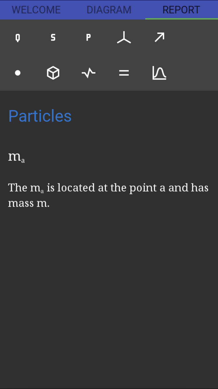
Create a particle

To complete the model, we must assign a mass to the point a. Return to the menu and tap the bodies panel, and then tap the plus sign to the left of the Particle line to open the "New Particle" dialog.

For the "ref_point_key" line, select the newly created point a, and for the mass select the parameter m. Tap the check button in the lower right, then close the menu dialog by tapping the menu button in the upper right. Returning to the diagram view, you will see the pendulum components have been added, including the newly created frame, vector, point, and mass.

Create the spring-damper

Lastly, we will expand the Loads panel in the menu, and tap the plus sign to create a New Translational Spring. The spring applies an equal and opposite force between two points in the mechanical system. Retain the default value of origin for the "start_point" in the dialog, and select the user-created point a for the "end_point." The previously-created stiffness, damping, and equilibrium length constants should be inserted into the corresponding line items "k," "c," and "equlibrium." Tap the check in the lower right to create the spring and complete the model. Tap in the upper right corner to close the menu, at which point you should see the diagram with the newly created particle and spring-damper.

Simulate

The hard part is over! To generate equations of motion, and simulate the dynamic response, simply tap the play button in the lower left corner of the diagram. Since this is a very simple model, the simulation will run nearly instantaneously. The animation will show the mass bouncing in the vertical direction with about a 1 second period, and gradually decaying to zero motion at an equilibrium position where the spring force balances the gravitational force.

Check out the report

Swipe right or tap on the the report tab in the upper right. Here you can view the settings you created earlier for generalized coordinates, parameters, points, and particles, as well as look at calculated equations, and plot the states as a function of time.

Next steps

• Experiment with mass, stiffness, damping, and initial position values
• Hint: tap the menu button with a pencil inside of a square to bring up the edit dialog for whichever component you want to modify
• Add a generalized speed, and initial vertical velocity
• Hint: use the generalized speed panel directly underneath the generalized coordinate panel
• Create a second mass-spring-damper stacked on top of the first
• Hint: repeat the same process of generating a vector, point, particle, and translational spring. Constants can be reused, generalized coordinates cannot.