
Introduction
The single-degree-of-freedom pendulum problem is likely the most common problem used to teach principles of mechanical engineering dynamics. This example shows how to use the "classic" interface in MOMDYN to define the kinematics of the pendulum problem, and simulate its response to a specified initial angle and angular velocity condition.Procedure
Using the classic interface, you will specify system constants (mass, and length of the pendulum), a single generalized coordinate (rotation angle), and use these to create a rotated reference frame, vector from the origin to the pendulum mass, a point, and a particle. At completion, you will simulate the oscillating pendulum and visualize it's dynamics.
Specify settings for the new model
Open MOMDYN, and tap once in the center of the screen to display the welcome screen. Tap the "Create" button, which will open the settings menu.


With the settings menu open, you can tap on each line item to bring up either a text input dialog, or a dropdown menu, for each respective item which can be used to modify their value, which is shown as the second text line for each item. Specify settings for the new model as follows:
- model_name: Pendulum
- model_description: Simple pendulum with a point mass and single angular degree of freedom
The "model_name" will be the name of the file if you choose to save the model. In this case, the saved pendulum model would display as user.Pendulum if you were to save and then tap the "Import" button on the welcome screen. The "model_description" is solely for informational purposes.
- gravity_method: Uniform
- gravity_constant: 9.8
- gravity_direction: -Y
Gravity can be modeled either as "None" or "Uniform," where in the latter case gravitational force on each body is equal to it's mass times the "gravity_constant" value. The gravitational force vector is given by the "gravity_direction" value.
- time_duration: 10.0
- simulation_rate: 100.0
The above values are used in simulation of the system. The "time_duration" in seconds is the total length of the simulation, and "simulation_rate" in Hertz (Hz) is the number of sample points per second in the output dataset if using a fixed-step solver , or initial step size if using an adaptive step solver.
The "simplify_equations" is useful for more complicated models, where trigonometric identities can be used to reduce the overall complexity, but tends to require more up-front computational time. The default "integration_method" is Runge-Kutta-Fehlberg (RKF45), and uses an adaptive step size with tolerance 0.001. Using smaller tolerances will generally reduce the step size and yield a more accurate simulation, but will increase computational time.
- simplify_equations: False
- integration_method: RKF45
- tol: 0.001
The "simplify_equations" is useful for more complicated models, where trigonometric identities can be used to reduce the overall complexity, but tends to require more up-front computational time. The default "integration_method" is Runge-Kutta-Fehlberg (RKF45), and uses an adaptive step size with tolerance 0.001. Using smaller tolerances will generally reduce the step size and yield a more accurate simulation, but will increase computational time.
Tap the "check" button in the lower right to close the settings menu and create the new model as-specified above.
Create parameters (constants)
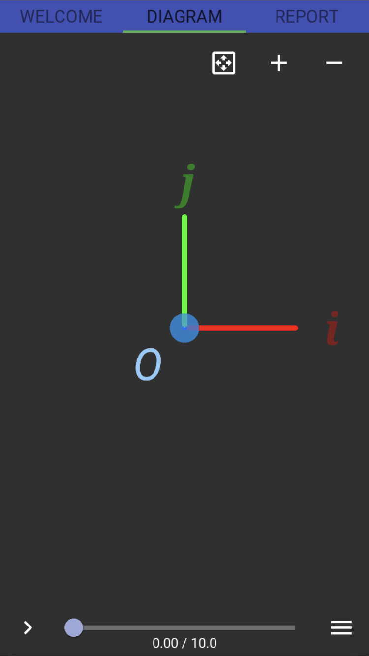
After closing the settings dialog, the screen will shift to the diagram view, with a single point representing the origin marked "O," and the inertial reference frame represented by the basis vectors (i, j, k).

Tap the menu button (three horizontal lines) in the lower right to obtain the menu dialog. Note the settings button in the upper left which will open the previous dialog, in case you want to edit any of the previously generated settings. The save button will save your model for future use, where it will be accessible using the import button on the first screen.
Tap on the panel labeled "Classic," which will expand to show several component options, each with four buttons, a "plus" to add, a "minus" to delete, a button to edit an existing component, and a question mark icon to view the help.
We will create parameters for the mass and length of the pendulum. Tap the plus symbol to open a "New Parameter" dialog. The "name" line item will be the symbol given to the parameter, The value is the numeric constant for that parameter, and the description is short text describing its usage. We will use the names "m" and "l" for mass and length, respectively. Enter 1 for each value. Descriptions are optional, but recommended to include, as I have done below.


Note that at this stage, if you close the menu dialog you will still only see the "blank slate" of the origin point and inertial frame. The parameter interface solely exists to create symbolic properties, they must later be assigned to their respective kinematic or dynamic objects, which is discussed in the sections to follow.
Create a generalized coordinate
Next we will create the generalized coordinate corresponding to the pendulum angle. Tap on the panel labeled "Generalized Coordinates," and then the plus sign on the left side. This will open the New Generalized Coordinate dialog.

Model the kinematics
Return to the menu and scroll down to see the "Frame," "Vector," and "Point" lines. We will be adding one of each of these.
Create a rotating reference frame
Tap the plus sign left of the frame line item to open the "New Frame" dialog.

Create vector from the origin to the mass
After returning to the menu, tap the plus sign left of the vector line to open the "New Vector" dialog.

The "name" line item for vectors corresponds to the label that will be displayed on top of the vector, but does not effect the equations of motion or simulation results. Likewise, the "start_point" line item represents the point from which the vector will originate in the diagram, but is strictly for visual purposes. Most importantly, the "ref_frame_key" and "x", "y," and "z" will define the vector as used in the back-end calculations. Each vector will have one or more dimensions, each measured in one of the three basis vectors associated with the specified frame. For the pendulum, select the newly created ref_frame_key = E, and the vector component x = l. This will generate a new vector designated r_0 = l*ex, where the name "r_0" is a default name given when None is provided by the user.
Create a point
Once again, return to the menu and tap the plus sign left of the point line to open the "New Point" dialog.

Points are positioned relative to an existing point using a vector as created above. Retain the default value for the "ref_point_key," which is the origin. Specify the newly created r_0 on the "vector_key" line. This will create a new point designated "a" which is a default name given when None is provided by the user.

Points are positioned relative to an existing point using a vector as created above. Retain the default value for the "ref_point_key," which is the origin. Specify the newly created r_0 on the "vector_key" line. This will create a new point designated "a" which is a default name given when None is provided by the user.
Create a particle
To complete the model, we must assign a mass to the point a. Return to the menu and tap the bodies panel, and then tap the plus sign to the left of the Particle line to open the "New Particle" dialog.


For the "ref_point_key" line, select the newly created point a, and for the mass select the parameter m. Tap the check button in the lower right, then close the menu dialog by tapping the menu button in the upper right. Returning to the diagram view, you will see the pendulum components have been added, including the newly created frame, vector, point, and mass.

Simulate the pendulum
The hard part is over! To generate equations of motion, and simulate the dynamic response, simply tap the play button in the lower left corner of the diagram. Since this is a very simple model, the simulation will run nearly instantaneously. The animation will show the pendulum swinging from right to left with around a 2.5 second period.
You'll notice that the animation is kind of jerky, why is that? Swipe right to get the report view, and then tap the button that looks like a graph to view the plot tab. Notice that the wave is coarsely sampled; the animation does a simple linear interpolation, so these coarse samples manifest as an animation that is not smooth.
You'll notice that the animation is kind of jerky, why is that? Swipe right to get the report view, and then tap the button that looks like a graph to view the plot tab. Notice that the wave is coarsely sampled; the animation does a simple linear interpolation, so these coarse samples manifest as an animation that is not smooth.
 |
| Simulated angle and rate for tol=0.001 |
Recall earlier when we created the model the setting for "tol" was 0.001. This is a fairly loose tolerance intended to get a fast result, but not the most accurate (you are on a mobile device after all, not a high-performance workstation). With the pendulum model, you can decrease this tolerance substantially and still get a fast calculation. Go back to the diagram view, then tap the edit menu button in the lower right, and settings button in the upper left of the edit dialog. Change the "tol" setting to 0.000001. Tap the check mark, return to the diagram view, and simulate once again. You will get a much smoother animation. Now go to the report view and plot tab, and note the much smoother wave form.
 |
| Simulated angle and rate for tol=0.000001 |
Next Steps
- Experiment with mass, length, and initial values
- Hint: tap the menu button with a pencil inside of a square to bring up the edit dialog for whichever component you want to modify.
- Add a generalized speed, and initial angular velocity
- Hint: use the generalized speed panel directly underneath the generalized coordinate panel
- Create a double pendulum
- Hint: repeat the same process of generating a frame, vector, point, and particle. Constants can be reused, generalized coordinates cannot.
No comments:
Post a Comment